This post is primarily directed at students in the AI class at University Erlangen to explain the Davis-Putnam (Logemann-Loveland) Algorithm for SAT solving and implication graphs for clause learning.
The goal in a SAT problem is to find an assignment that satisfies a set of propositional formulae \( \Delta\), or a proof that none exist, i.e. that the set is unsatisfiable. DPLL is closely related to the resolution calculus, and as with resolution we first transform \( \Delta\) to a set of clauses \( \Delta=\{L_1, \ldots, L_n\}\), where each clause \( L_i\) is a set of literals \( L_i=\{ \ell_{i1}, \ldots, \ell_{in_i}\}\), where a literal \( \ell\) is either a propositional variable or the negation of a propositional variable. We write \( \ell=A^T\) if \( \ell\) is the propositional variable \( A\) and \( \ell=A^F\) if it is the negation of \( A\). Then \( \Delta\) corresponds to the formula
\[\displaystyle\bigwedge_{L\in\Delta}\bigvee_{\ell\in L}\ell=\bigwedge_{i=1}^n\bigvee_{j=1}^{n_i}\ell_{ij}\]
in conjunctive normal form (CNF).
The basic algorithm \( \textsf{DPLL}\) takes a clause set \( \Delta\) and a partial assignment \( I: V\to\{0,1\}\) (where \( V\) is the set of propositional variables) as arguments (starting with the empty assignment) and returns either a partial assignment that satisfies \( \Delta\) or \( \textsf{unsatisfiable}\) if none exist. It proceeds as follows:
- Unit Propagation: If \( \Delta\) contains a unit, that is a clause \( L=\{ \ell \}\) with just one literal, then we extend our current assignment by that literal; meaning if \( L=\{ A^T \}\), then we let \( I(A)=1\) and if \( L=\{ A^F \}\) we let \( I(A)=0\). Then we simplify (more on that later) \( \Delta\) with our new assignment and repeat.
- When \( \Delta\) contains no units anymore, we check whether \( \Delta\) is now empty; if so, we are done and we return our current assignment \( I\). If not, we check whether \( \Delta\) now contains an empty clause; if so, we return \( \textsf{unsatisfiable}\).
- Splitting: So \( \Delta\) now is not empty, contains no empty clauses and contains no units. We’re left with guessing an assignment, so we pick one propositional variable \( A\) on which our assignment \( I\) is currently undefined, let \( I(A)=1\), simplify \( \Delta\) with our new assignment and recurse. If \( \textsf{DPLL}(\Delta,I)\) returns an assignment, that means we guessed currently and we return that. If it returns \( \textsf{unsatisfiable}\), we guessed wrong and instead let \( I(A)=0\), simplify and recurse with that.
- By simplify I mean: If in our current assignment we have \( I(A)=1\) (or \( I(A)=0\) respectively), then we delete from \( \Delta\) all clauses that contain the literal \( A^T\) (respectively \( A^F\)). In the remaining clauses, we eliminate the literal \( A^F\) (respectively \( A^T\)).
Now why does this work? Let’s start with unit propagation: If \( \Delta\) contains a unit literal \( \{ A^T \}\), then the formula corresponding to our clause set looks like this: \[\displaystyle L_1\wedge\ldots\wedge L_n\wedge A\] and obviously, for this formula to be satisfied, we need to set \( I(A)=1\). Conversely, if we have the unit literal \( \{ A^F \}\), then the formula looks like this: \[\displaystyle L_1\wedge\ldots\wedge L_n\wedge \neg A\] and we obviously need to set \( I(A)=0\) to satisfy \( \Delta\). Now for simplification: If we assign \( I(A)=1\), then any clause that contains the literal \( A^T\) will be satisfied by \( I\), since clauses are interpreted as the disjunction of its literals. Consequently, we can ignore these clauses from now on. The remaining clauses however will still need to be satisfied, and if we have \( I(A)=1\), then we know that the literal \( A^F\) will be false anyway, which means we can ignore it in any disjunction (i.e. clause) containing it.
Example: Let \( \Delta = \{ \{P^F, Q^F, R^T\}, \{P^F,Q^F,R^F\}, \{ P^F, Q^T, R^T\}, \{P^F, Q^T, R^F\} \}\). Then \( \textsf{DPLL}(\Delta,\{\})\) proceeds like this:
- We have no unit clauses, our assignment is empty, no clause is empty and \( \Delta\) isn’t empty, so we can only split. We pick the variable \( P\):
- We let \( I(P)=1\) and simplify, yielding \( \Delta_1 = \{ \{Q^F, R^T\}, \{Q^F, R^F\}, \{Q^T, R^T\}, \{Q^T, R^F\} \}\). We have no unit clauses, no clause is empty and \( \Delta_1\) isn’t empty, so we can only split. We pick the variable \( Q\):
- We let \( I(Q)=1\) and simplify, yielding \( \Delta_2 = \{ \{R^T\}, \{R^F\} \}\). We have a unit clause, so we do unit propagation by letting \( I(R)=1\) and simplifying. Unfortunately, that yields \( \Delta_3=\{ \{\} \}\) containing the empty clause, so we return \( \textsf{unsatisfiable}\).
- Since the former branch failed, we let \( I(Q)=0\) and simplify, yielding \( \Delta_2 = \{ \{R^T\}, \{R^F\} \}\). We have a unit clause, so we do unit propagation by letting \( I(R)=1\) and simplifying. Again, that yields \( \Delta_3=\{ \{\} \}\) containing the empty clause, so we return \( \textsf{unsatisfiable}\)
- The former branch failed, so we let \( I(P)=0\) and simplify, yielding \( \Delta_1 = \{\}\). \( \Delta_1\) is empty, so we return the current assignment \( I=\{P\to0\}\).
- We let \( I(P)=1\) and simplify, yielding \( \Delta_1 = \{ \{Q^F, R^T\}, \{Q^F, R^F\}, \{Q^T, R^T\}, \{Q^T, R^F\} \}\). We have no unit clauses, no clause is empty and \( \Delta_1\) isn’t empty, so we can only split. We pick the variable \( Q\):
Apart from unit propagation and simplification, all that \( \textsf{DPLL}\) does is guessing assignments and backtracking if it fails. As such, it can very easily happen that the algorithm tries the same failing partial assignment again and again; e.g. because somewhere along the way it splits on a propositional variable that has nothing to do with why it failed before. A nice example of how this can happen is, if we have basically independent clauses that don’t share any propositional variables in the first place:
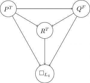
Example: We take the clause set from before and pointlessly extend it by the independent clauses \( \{ X_1^T, \ldots, X_{100}^T \}\) and \( \{ X_1^F, \ldots, X_{100}^F \}\). Obviously, these are basically two independent SAT problems that don’t share any propositional variables. But as we’ve seen before, if we start with \( I(P)=1\) our original clause set will necessarily fail, but the algorithm will only notice once \( Q\) (and \( R\)) have been assigned as well. If our \( \textsf{DPLL}\) run will start with \( P=1\), but (in the worst case) then continue with \( X_1,\ldots X_{100}\) first, it will try the same assignments for \( Q\) and \( R\) again and again:
This is where clause learning comes into play: If we fail, we want to figure out why we failed and make sure we don’t make the same mistake all over again. One way to do this is with implication graphs, that systematically capture which chosen assignments lead to a contradiction (or imply which other assignments via unit propagation). An implication graph is a directed graph whose nodes are literals and the symbols \( \Box_L\) (representing the clause \( L\) becoming empty, i.e. a failed attempt). We construct such a graph during runtime of \( \textsf{DPLL}\):
- If at any point a clause \( L=\{\ell_1,\ldots,\ell_n, u\}\) becomes the unit clause \( \{ u \}\), then for each literal \( \ell\in L\) with \( \ell\neq u\) we add an edge from \( \overline{\ell}\) to \( u\) (where \( \overline \ell\) is the negation of the literal \( \ell\)).
The intuition behind this being, that when we do unit propagation, we’re using the fact the formula \( \ell_1 \vee \ldots \vee \ell_n \vee u\) is logically equivalent to \( (\overline{\ell_1} \wedge \ldots \wedge \overline{\ell_n}) \to u\). The new edge is (sort-of) supposed to capture this implication. - If at any point a clause \( L=\{\ell_1,\ldots,\ell_n\}\) becomes empty, then for each literal \( \ell\in L\) we add an edge from \( \overline{\ell}\) to \( \Box_L\).
Here we are using the fact, that the formula \( \ell_1 \vee \ldots \vee \ell_n\) is logically equivalent to \( (\overline{\ell_1} \wedge \ldots \wedge \overline{\ell_n}) \to \bot\).
Before we answer the question why we’re doing this, let’s go back to our previous example and construct the implication graph to the first contradiction. To keep track of which clause a literal is coming from, let’s name them:
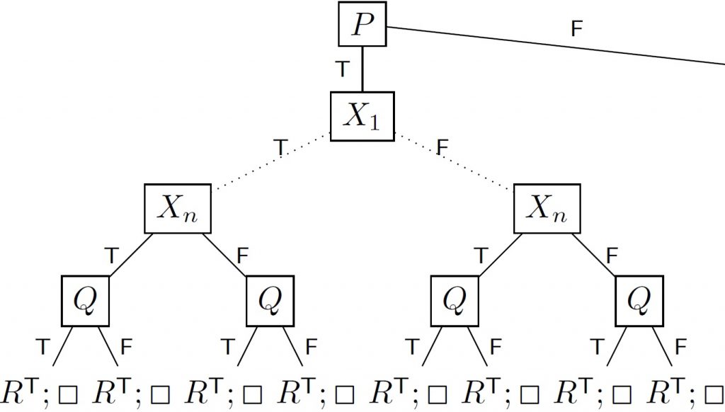
Example: Let again \( \Delta = \{ L_1, L_2, L_3, L_4 \}\) where \( L_1=\{P^F, Q^F, R^T\}\), \( L_2=\{P^F,Q^F,R^F\}\), \( L_3=\{ P^F, Q^T, R^T\}\) and \( L_4=\{P^F, Q^T, R^F\} \}\). Then \( \textsf{DPLL}(\Delta,\{\})\) proceeds like this:
- We start by splitting at the variable \( P\):
- We let \( I(P)=1\) and simplify, yielding \( \Delta_1 = \{ L_1=\{Q^F, R^T\}, L_2=\{Q^F, R^F\}, L_3=\{Q^T, R^T\}, L_4=\{Q^T, R^F\} \}\). Then we split at the variable \( Q\):
- We let \( I(Q)=1\) and simplify, yielding \( \Delta_2 = \{ L_1=\{R^T\}, L_2=\{R^F\} \}\). \( L_1\) is now a unit clause. Apart from \( R^T\), the original \( L_1\) also contained the literals \( P^F\) and \( Q^F\), so we add to our graph two new edges to \( R^T\), one from \( P^T\) and one from \( Q^T\) (remember: from the negations of the original literals!).Now we do unit propagation , resulting in \( L_2\) becoming the empty clause. The original \( L_2\) contained the literals \( P^F\), \( Q^F\) and \( R^F\), so we add edges from \( P^T\), \( Q^T\) and \( R^T\) to \( \Box_{L_2}\) and return \( \textsf{unsatisfiable}\).
- We let \( I(P)=1\) and simplify, yielding \( \Delta_1 = \{ L_1=\{Q^F, R^T\}, L_2=\{Q^F, R^F\}, L_3=\{Q^T, R^T\}, L_4=\{Q^T, R^F\} \}\). Then we split at the variable \( Q\):
The resulting graph looks like this:
So, how does that help? Well, the graph tells us pretty straight, which decisions lead to the contradiction, namely \( P^T\), \( Q^T\) and \( R^T\). But more than that, it tells us that \( R^T\) wasn’t actually a decision; it was implied by the other two choices. So in our next attempt, we need to make sure we don’t set \( P\) and \( Q\) to \( 1\). The easiest way to do that is to add a new clause for \( \neg (P \wedge Q)\), which is \( Ln_1=\{ P^F, Q^F \}\). Hooray, we learned a new clause! Before we examine how exactly we construct clauses out of graphs, let’s continue our example with this newly added clause:
Example continued:
- –
- –
- –
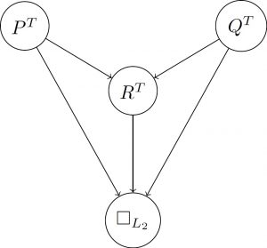
- Since the former branch failed, we add our new clause and simplify, yielding \( \Delta_1 = \{ L_1=\{Q^F, R^T\}, L_2=\{Q^F, R^F\}, L_3=\{Q^T, R^T\}, L_4=\{Q^T, R^F\}, Ln_1=\{Q^F\} \}\). Now \( Ln_1\) became a unit clause, so we add an edge from \( P^T\) to \( Q^F\), do unit propagation by letting \( I(Q)=0\) and simplify, yielding \( \Delta_2 = \{ L_3=\{R^T\}, L_4=\{R^F\} \}\).
Now \( L_3\) became a unit, so we need to add edges from \( P^T\) and \( Q^F\) to \( R^T\).We do unit propagation again and \( L_4\) becomes the empty clause, adding the edges from \( P^T\), \( Q^F\) and \( R^T\) to \( \Box_{L_4}\). Finally, we return \( \textsf{unsatisfiable}\).
- –
The resulting graph:
This time, we can immediately see that the bad choice was \( P^T\). We can learn from this, by adding the new clause \( Ln_2=\{ P^F \}\), which of course is a unit and thus immediately becomes part of our assignment.
So, how exactly do we get from implication graphs to clauses? That’s simple: starting from the contradiction we arrived at, we take every ancestor of the \( \Box\)-node with no incoming edges – i.e. the roots. Those are the literals that were chosen during a split-step in the algorithm, and the other ancestors are all implied (via unit propagation) necessarily by those choices. These choices (i.e. their conjunction) lead to the problem, so we take their negation and add them as a new clause: In the first example graph, the roots were the node \( P^T\) and \( Q^T\), so we added the new clause \( \{ P^F, Q^F \}\). In the second graph, the only root was \( P^T\), so we added the clause \( \{ P^F \}\).
Admittedly, in this example adding the learned clauses didn’t actually help much – but imagine bringing the variables \( X_1,\ldots,X_{100}\) back into the mix. Where we had hundreds of almost identical branches before, with clause learning the search tree of the algorithm will look more like this:
Two failures are now enough to conclude, that setting \( I(P)=1\) was already a mistake and we can immediately backtrack to the beginning.